Unraveling Complexity: Network Science Applied to Star Wars Films
This blog post explores the fundamentals of Network Analysis using the Star Wars character interactions.
Introduction
In our world, everything is connected - from the neurons firing in your brain to the spread of a viral tweet. This interconnectedness isn’t limited to our reality; it extends to the fictional realms we create. The Star Wars universe, with its rich tapestry of characters and their interactions, provides a perfect backdrop for exploring the world of network analysis.
What are Networks?
Networks are the invisible architecture of our world - structures of interconnected elements that offer a lens for understanding complex systems. These intricate webs of relationships reveal patterns and behaviors that span from the microscopic to the societal. The study of networks, often referred to as network science, has emerged as a powerful tool for understanding complex systems across various domains. By analyzing the structure and dynamics of networks, researchers can uncover hidden patterns, predict emergent behaviors, and design more efficient and resilient systems.
In the physical sciences, networks can model the spread of infectious diseases, illustrating how pathogens navigate through populations
Each node and connection tells a story, from how ideas propagate, how disease spreads, to how social movements emerge. In this blog post, I dive into the fascinating world of network analysis, exploring its applications, methodologies, and the insights it offers using a dataset of Star Wars character interactions to demonstrate these concepts.
Network Science Fundamentals
Before delving into the Star Wars dataset, it is helpful to understand the fundamental concepts of network analysis such understanding how various elements are related, how connected they are to other elements, and how central they are to the network as a whole.
Structure
At its core, a network (also known as a graph) is a representation of connections among a set of items. The building blocks of any network are nodes (or vertices) and edges (or links or ties). Nodes represent the items or entities in our network - in a social network, these might be people, while in a computer network, they could be devices. Edges, on the other hand, represent the connections between these nodes. In our social network example, an edge might signify a friendship between two people.
Not all networks are created equal, however. The nature of relationships in a network can vary, leading to different types of structures. Networks can be symmetric or asymmetric. Symmetric networks, like friendships or family ties, have reciprocal relationships - if Alice considers Bob a friend, Bob typically considers Alice a friend too. Asymmetric networks, such as food webs, have one-way relationships - a lion eats a zebra, but the zebra certainly doesn’t eat the lion! This concept of symmetry leads us to another important distinction: directed versus undirected networks. Undirected networks are used for symmetric relationships where edges have no direction, while directed networks are perfect for asymmetric relationships, with edges having a clear source and destination.
Real-world relationships often have more nuance than a simple “connected or not” binary, which brings us to the concepts of weighted networks and multigraphs. In a weighted network, edges carry numerical values to represent the strength or intensity of a relationship. For instance, in a friendship network, your best friend might have an edge weight of 10, while an acquaintance might only rate a 2. Multigraphs take this complexity a step further, allowing for multiple edges between the same pair of nodes. This is useful when a single type of connection isn’t enough to capture the full nature of a relationship. For example, two people might be simultaneously coworkers, neighbors, and members of the same book club.
Degree
In network analysis, the concept of “degree” is fundamental to understanding the connectivity and structure of graphs. For undirected graphs, the degree of a node is simply the number of edges connected to it, representing the count of its immediate neighbors. This is often denoted as $deg(v)$ for a node $v$. The degree distribution of a graph provides a broader view of connectivity, representing the probability distribution of degrees across the entire network. This distribution is crucial for understanding the overall structure and characteristics of the network, such as in scale-free networks where it often follows a power law.
When dealing with directed graphs, we need to consider the direction of the edges, which leads to two types of degree: in-degree and out-degree. The in-degree, often denoted as $deg⁻(v)$, represents the number of edges pointing towards the node, while the out-degree, denoted as $deg⁺(v)$, represents the number of edges pointing away from the node. For example, in a citation network, a paper’s in-degree would represent how many times it has been cited, while its out-degree would indicate how many other papers it cites. When analyzing directed graphs, we consider separate distributions for in-degree and out-degree, which can reveal important characteristics of the network, such as the presence of hubs (nodes with unusually high in-degree or out-degree) or overall connectivity patterns.
Understanding degree and degree distributions is crucial in network analysis for several reasons. It helps identify important or influential nodes, provides insights into the network’s resilience and vulnerability, aids in comparing different networks and understanding their structural properties, and can reveal underlying processes that govern the network’s formation and evolution.
| Degree | Probability |
|---|---|
| 1 | 1/9 |
| 2 | 4/9 |
| 3 | 1/3 |
| 4 | 1/9 |
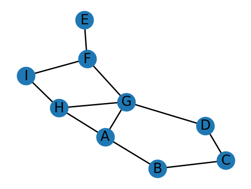
This network consists of 9 nodes, each with varying numbers of connections (degrees). The degree distribution is as follows: One-Degree Nodes: There is only one node with a single connection, representing a probability of 1/9 (approximately 11.1%) for a randomly selected node to have one degree. Two-Degree Nodes: Four nodes have two connections each. This means the probability of randomly selecting a two-degree node is 4/9 (approximately 44.4%). Other Degrees: The remaining four nodes have varying degrees, which can be calculated similarly. This distribution provides insights into the network's structure, showing that two-degree nodes are the most common in this particular network.
Connectivity
In network analysis, one of the most fundamental questions we ask is whether every node of the network can reach every other node. This concept is known as connectivity. A network is considered connected if there’s a path between any two nodes. In simpler terms, in a connected network, you can start at any point and find a way to reach any other point by following the edges (connections) between nodes.
However, not all networks are fully connected. When a network isn’t completely connected, we can identify distinct groups within it. These groups are called connected components. Each component is like a mini-network within the larger network. Within a component, every node can reach every other node, but nodes in one component cannot reach nodes in other components.
A network that is not connected can be divided into distinct, self-contained groups of nodes called connected components. Each connected component represents a subset of the network where every node within the component has a path to every other node within the component, but this property does not hold true for a larger set of nodes (i.e., not fully connected to a larger piece of the graph).
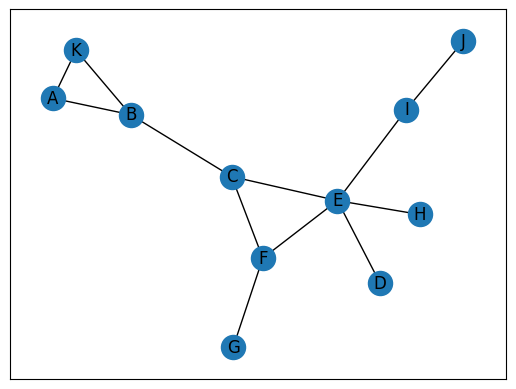
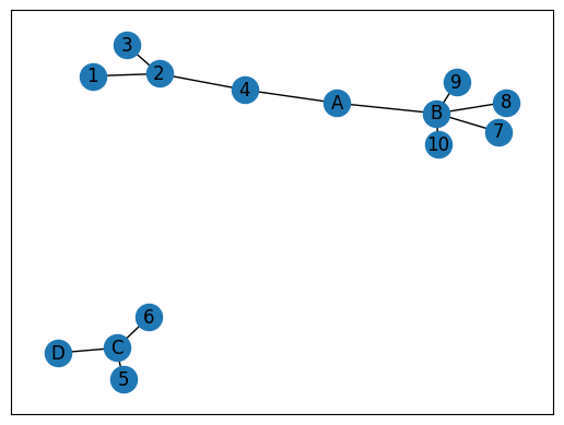
(Left) Connected Network: This graph demonstrates a fully connected network. Every node (represented by circles) can reach every other node by following a path along the edges (lines) that connect them. For instance, we can trace a path from node A to node J by following the sequence A-B-C-E-I-J. This illustrates the concept of complete connectivity within a network. (Right) Disconnected Network: This image shows a disconnected network comprising two separate components. Within each component, nodes are interconnected, but there are no paths between nodes in different components. For example, there is no way to travel from node D to node A, as they belong to distinct, isolated parts of the network. This demonstrates the concept of partial connectivity and the existence of multiple components within a single network structure.
Understanding the connectivity of a network is crucial for several reasons. It helps us identify isolated groups or subcultures in social networks, detect potential communication breakdowns in organizational structures, and analyze the robustness of systems, such as how easily information or diseases can spread. By examining both the overall connectivity and the specific structures within connected components, we can gain valuable insights into the dynamics and behavior of complex networks across various domains
Distance
Beyond simple connectivity, it’s often more informative to quantify the distance between nodes. For example, in the spread of news, understanding how many “hops” information must take to travel between individuals is vital.
The distance between two nodes is defined as the length of the shortest path between them, where each step along a path represents a connection between nodes. We can then characterize the distance between all pairs of nodes in a graph by looking at the average distance between every pair of nodes in the network or the maximum distance between any pair of nodes. We can look at the average distance between all pairs of nodes to understand how “tight-knit” a network is. The maximum distance (or diameter) tells us the “width” of our network.
Breadth-first search (BFS) is a common algorithm used to efficiently find shortest paths in networks. The algorithm is as follows:
- Find all distances to a seed node.
- Find all connections to the seed node and declare them to be at distance 1.
- For each node found in step 1, find all their connections which were not previously found, and declare them to be at distance 2.
- Continue discovering new nodes in layers with each new layer adding one to the distance.
| Distance | Nodes |
|---|---|
| 1 | K, B |
| 2 | C |
| 3 | E, F |
| 4 | H, I, D, G |
| 5 | J |
Centrality
Centrality is a fundamental concept in network analysis that aims to identify the most important or influential nodes (vertices) within a network. It essentially helps answer the question: “Which nodes are the key players in this network?” Centrality measures quantify the importance of nodes based on their position in the network, with different measures capturing various aspects of importance or influence. The choice of centrality measure depends on the specific context and research questions at hand.
Common centrality measures include degree centrality, which looks at the number of connections a node has; closeness centrality, which measures how easily a node can reach all other nodes; betweenness centrality, which gauges how often a node acts as a bridge between other nodes; and eigenvector centrality, which considers the importance of a node’s connections. These measures help researchers and analysts understand which nodes play crucial roles in a network’s structure and function, which can be invaluable for identifying key influencers, bottlenecks, or vulnerable points in a system.
There are various centrality measures, below is a summary of the common ones:
| Centrality Measure | Assumptions | Formula |
|---|---|---|
| Degree centrality | Important nodes have many connections. | Undirected: $C_D(v) = \frac{deg(v)}{n - 1}$ where $n$ is the number of nodes in the network and $deg(v)$ is the degree of node $v$. Directed: $C_{D}^{in}(v) = \frac{deg^{in}(v)}{n - 1}$ $C_{D}^{out}(v) = \frac{deg^{out}(v)}{n - 1}$ where $deg^{in}(v)$ is the in-degree of node $v$ (number of edges pointing to $v$) and $deg^{out}(v)$ is the out-degree of node $v$ (number of edges pointing from $v$ to other nodes). |
| Closeness centrality | Important nodes are close to other nodes. | $C_C(v) = \frac{n - 1}{\sum_{u \in V \setminus {v}} d(v,u)}$ where $n$ is the total number of nodes in the network, $V$ is the set of all nodes in the network, and $d(v,u)$ is the shortest path distance between nodes $v$ and $u$. |
| Betweenness centrality | Important nodes act as bridges between other nodes. | $C_B(v) = \sum_{s \neq v \neq t} \frac{\sigma_{st}(v)}{\sigma_{st}}$ where $s$ and $t$ are nodes in the network different from $v$, $\sigma_{st}$ is the total number of shortest paths from node $s$ to node $t$, and $\sigma_{st}(v)$ is the number of those paths that pass through $v$. [1] |
- For undirected graphs: $\frac{1}{2}(\lvert N \rvert - 1)(\lvert N \rvert - 2)$
- For directed graphs: $(\lvert N \rvert - 1)(\lvert N \rvert - 2)$
Where $\lvert N \rvert$ is the number of nodes in the network.
With this overview of the fundamentals of network analysis, we have enough information to begin our exploration into the Star Wars character interactions.
Star Wars Network Analysis: A Case Study
In this blog post, I will embark on a data-driven journey through the Star Wars galaxy. We’ll use network analysis to:
- Identify the most central characters in the Star Wars universe
- Uncover hidden communities and alliances
- Visualize the complex web of relationships across different films
- Predict potential plot points based on network structures
Whether you’re a die-hard Star Wars fan, a data science enthusiast, or just curious about how stories are structured, this analysis will offer new insights into both network science and the galaxy far, far away. If you would like to reference the code used for this blog, you may reference the notebook in my public blogs GitHub repository.
Data Source
The network data we’ll be using for this analysis is based on the work of Evelina Gabasova. She extracted interactions between characters from the scripts of Star Wars Episodes I through VII. The network is defined by characters who speak to each other within the same scene where the nodes are the characters and the edges represent their communication. The network is undirected and the edges are weighted by the number of interactions between the characters.
You can find the code used to create the network on GitHub and download the data itself from Kaggle
Exploratory Analysis
=== Network Summary ===
Number of characters:                    110
Number of interactions:                  398
Number of connected components:          2
Number of isolated nodes:                1

=== Network Structure Insights ===
Network density:                         0.0664
Average clustering coefficient:          0.6768

=== Interaction Details ===
Character with the most interactions:    ANAKIN (41 interactions)
Character with the least interactions:   GOLD FIVE (0 interactions)
Average number of interactions:          7.24
Standard deviation of interactions:      7.73

=== Centrality Measures ===
Character with highest degree centrality: ANAKIN (0.3761)
Character with lowest degree centrality: GOLD FIVE (0.0000)
Character with highest betweenness centrality: OBI-WAN (0.2129)
Character with lowest betweenness centrality: PK-4 (0.0000)
Character with highest closeness centrality: OBI-WAN (0.5516)
Character with lowest closeness centrality: GOLD FIVE (0.0000)

=== Clustering Measures ===
Average clustering coefficient:          0.6768
Transitivity:                            0.3490

=== Path Analysis ===
Network is not connected; average shortest path length and diameter are not defined.