Predicting Top 10 Formula 1 Finishes and Clustering Race Tracks
This project uses machine learning to predict top 10 finishes in F1 races and cluster tracks by characteristics.

Introduction
Formula 1, often hailed as the pinnacle of motorsport, combines high-speed competition, cutting-edge technology, and a global fan base. This premier racing series showcases a unique synergy of engineering excellence, driver skill, and strategic depth, making it an intriguing subject for in-depth analysis. This project leverages machine learning to explore the complexities of Formula 1, with a primary focus on predicting top 10 finishes in races — a crucial outcome for securing championship points for drivers and teams. Additionally, we analyze race track characteristics through unsupervised learning, clustering tracks based on factors such as layout, surface, and length.
Historically, Formula 1 analytics has focused on predicting race winners using various statistical and machine learning techniques. These studies often reflect the dominance of certain teams during specific eras, such as Red Bull’s supremacy from 2010 to 2013 and 2021 to the present, and Mercedes’ stronghold from 2013 to 2020. While insightful, this focus on predicting race winners can overlook the nuanced dynamics and strategic elements that contribute to the broader competitive landscape of Formula 1 racing.
Our project aims to broaden the analytical scope by targeting the prediction of top 10 finishes. Securing a place in the top 10 is vital for accumulating championship points, crucial for both drivers and constructors over a season. By shifting our focus to these positions, we aim to capture the intricate competitive interactions and strategic nuances that influence race outcomes beyond the winner’s podium. This approach provides a more comprehensive understanding of performance determinants in Formula 1, addressing both the predictability associated with team dominance and the variability arising from tactical decisions across the grid.
The Formula 1 points system awards points to the top 10 finishers in a grand prix, with the winner receiving 25 points, second place 18 points, and so on down to 1 point for the 10th place. Additionally, there is a bonus point for the fastest lap (FL) in the grand prix, provided the driver finishes in the top 10. In the shorter sprint races – about one-third the distance of a typical Grand Prix distance – points are awarded to the top 8 finishers, with the winner getting 8 points. This system, in place since 2010, was designed to create a larger gap between first and second place and to accommodate the expanded grid and improved reliability of modern cars.
| Position | 1st | 2nd | 3rd | 4th | 5th | 6th | 7th | 8th | 9th | 10th | FL |
|---|---|---|---|---|---|---|---|---|---|---|---|
| Points | 25 | 18 | 15 | 12 | 10 | 8 | 6 | 4 | 2 | 1 | 1 |
Additionally, our exploration into the unsupervised clustering of race tracks adds another dimension to this analysis. By uncovering similarities and distinctions among tracks, we offer deeper insights into how different track characteristics influence racing strategies and outcomes. This dual-faceted approach distinguishes our work from conventional race prediction analyses, offering a novel perspective on the dynamics of Formula 1 racing.
Data Source
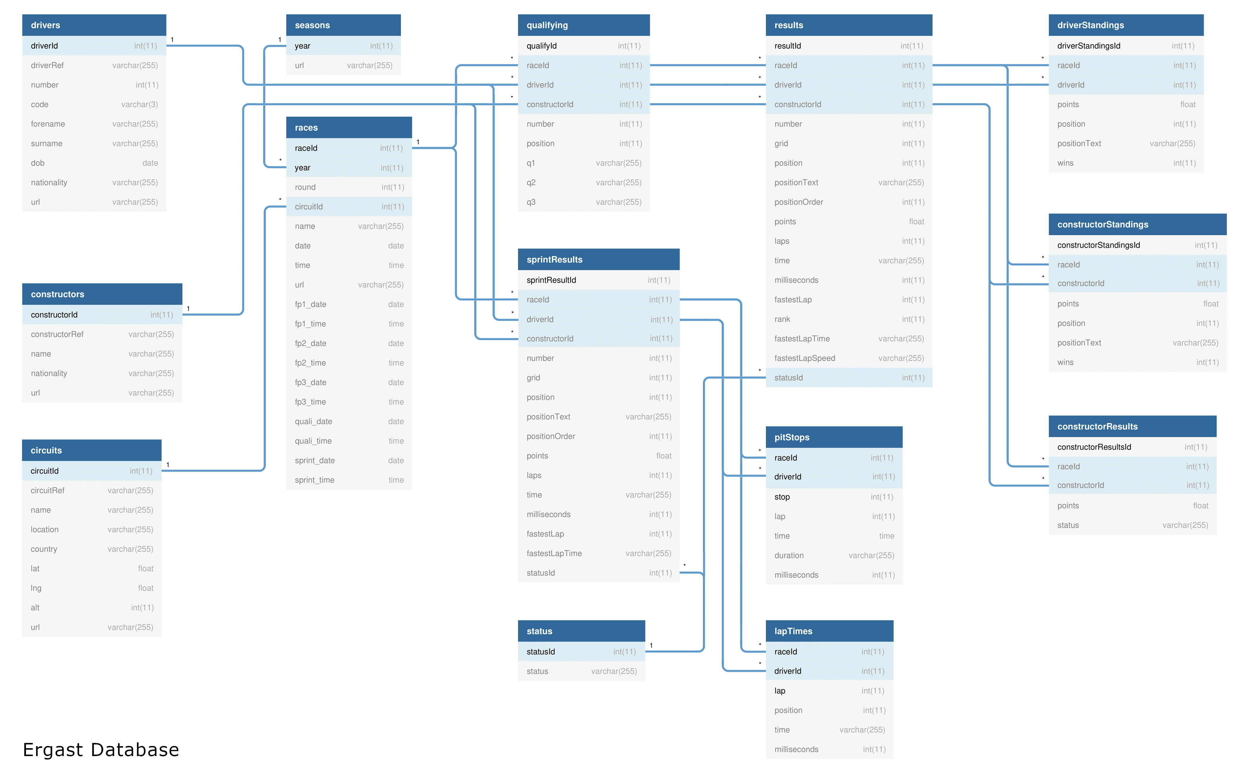
The Ergast Developer API serves as a pivotal data source for our Formula 1 analysis, offering an extensive repository of historical race data, including driver standings, race results, and qualifying times
Reproducibility Note
The public Ergast API is set to sunset after the 2024 formula 1 season. To recreate You can find legacy data on Kaggle or in this project’s GitHub repository.
Preprocessing
Top 10 Predictions
To prepare the dataset for supervised learning, a pre-processing routine was implemented, focusing on extracting and structuring key information from the Ergast Developer API. Initially, unique identifiers for races and racers were constructed using a combination of the race year and session for RaceId, and a concatenation of the racer’s first and last names for RacerId. These identifiers serve as indexes to uniquely identify data points without directly contributing to the model’s input features. For the Type of track, we categorized circuits into purpose-built tracks and street circuits, encoded as 0 and 1, respectively, based on circuit information obtained from the API. This binary classification aids the model in distinguishing the inherent differences between these track types. Additionally, we derived the TrackId by using the circuit name, ensuring a consistent reference across different datasets. The previous year’s race result for each racer, Qualifying position, and the timings for Q1, Q2, and Q3 were meticulously extracted and formatted, with non-participation or non-qualification explicitly marked, ensuring a comprehensive dataset ready for analysis.
| Column Name | Description | Type |
|---|---|---|
| RaceId | Year-Session (e.g., 2021-Bahrain) | Index |
| RacerId | First name-Last name (e.g., Lewis-Hamilton) | Index |
| TrackId | Circuit name (e.g., Silverstone) | Index |
| Previous year result | Racer's previous year result (0 if not available) | Feature |
| Qualifying position | Racer's qualifying position | Feature |
| Q1 timing | Qualifying round 1 timing | Feature |
| Q2 timing | Qualifying round 2 timing (0 if did not qualify for Q2) | Feature |
| Q3 timing | Qualifying round 3 timing (0 if did not qualify for Q3) | Feature |
| Race finish | Race finish position | Label |
Track Clustering
Our clustering of circuits based on track characteristics provides insight into how tracks relate to one another across a number of characteristics. We employed unsupervised learning techniques to uncover latent groupings among F1 circuits worldwide.
For our analysis of F1 track characteristics, we leveraged three data sources. The first was a table of F1 track characteristics scraped from wikipedia. The second was a track characteristic retrieved from the Ergast API. The third was a dataset of F1 circuits from Kaggle. Details of the data sources are provided in the table below.
| Attribute | Wikipedia | Ergast API | Kaggle |
|---|---|---|---|
| Location | Wikipedia List of F1 Circuits | API Queryhttps://ergast.com/api/f1/circuits?limit=100&offset=0 was used as the API endpoint. However, note that the API service is deprecated as of 2024. | Kaggle F1 circuits.csv dataset |
| Format | scraped html table | JSON | CSV |
| Important Variables Included | Circuit Name, Type, Direction, circuit length in kilometers | circuit name, altitude | Number of turns |
| Number of records | 77 | 77 | 80 |
| Time Period Covered | 1950-2023 | 1950-2023 | 1950-2023 |
| Preprocessing | Extract track length from text string, convert to numeric | Match track names from the Wikipedia table using Levenshtein distance, and perform a left join with the Wikipedia data. | Match track names from the Wikipedia table using Levenshtein distance, and perform a left join with the Wikipedia data. . Impute missing number of turn values with K nearest neighbors imputer. |
After our initial data sourcing and preprocessing, we developed a dataset that contained 5 complete features for all 77 F1 circuits since 1950: altitude, track length in kilometers, number of turns, circuit type (road, race, or street), and circuit direction (clockwise, counterclockwise, or figure eight). Our selection of features to represent circuits was informed by consultations with F1 enthusiasts, ensuring our analysis represented how F1 subject matter experts would evaluate and characterize tracks.
Exploratory Data Analysis
Our data analysis phase utilized a suite of visual tools to dissect and understand the underlying patterns within the Formula 1 dataset. Through the use of heatmaps, we were able to discern the correlation across various features, providing us with an initial glimpse into the relationships between variables such as qualifying times, previous year’s positions, and their impact on race outcomes. Pair plots further enriched our analysis by offering a granular view of the pairwise relationships between features, revealing trends, clusters, and potential outliers that could influence model performance. Additionally, leveraging feature importance plots, particularly from our Random Forest model, allowed us to identify the most predictive variables in determining top 10 finishes. This visual exploration not only guided our feature selection process but also offered profound insights into the factors that most significantly affect race performance, laying a robust foundation for our predictive modeling efforts. This comprehensive approach to data analysis ensures that our models are built on a nuanced understanding of the dataset, maximizing their ability to uncover meaningful patterns and predictions.
Multivariate Analysis
A heatmap is a graphical representation of data where values are depicted by color, allowing for an intuitive perception of patterns, such as correlations between variables in a dataset, which can be crucial for identifying relationships and trends at a glance.
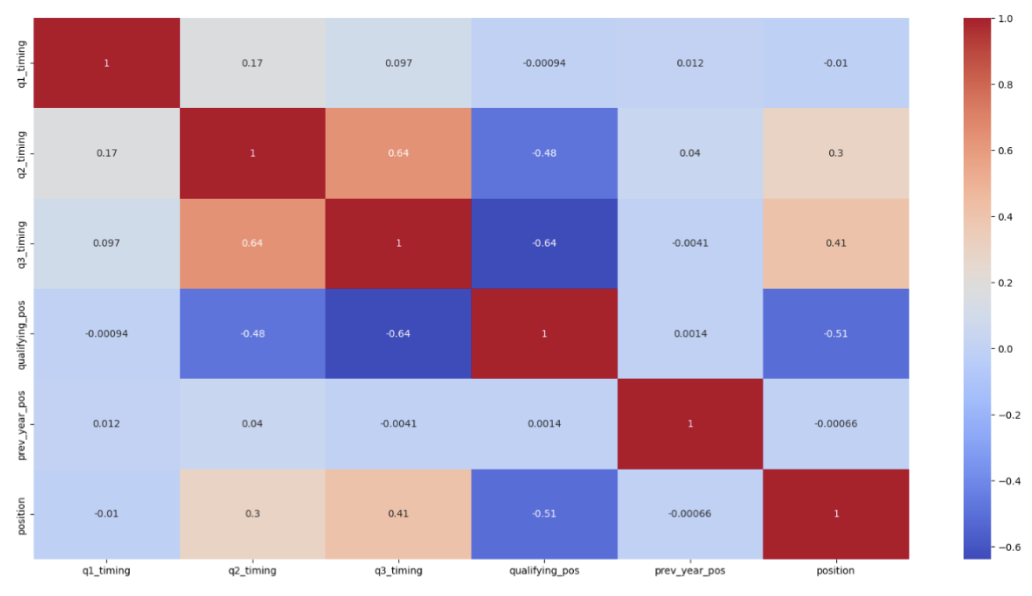
- Strong Negative Correlation between Qualifying Position and Race Position: There is a strong negative correlation (r = -0.51) between
qualifying_posandposition. This suggests that drivers with better (lower number) qualifying positions tend to finish the race in better (also, numerically lower) positions. - Positive Correlation between Q2 and Q3 Timings: The
q2_timingandq3_timinghave a strong positive correlation (r = 0.64). This indicates that drivers who perform well in Q2 also tend to perform well in Q3. - Negative Correlation between Q2/Q3 Timings and Qualifying Position: Both
q2_timingandq3_timingshow a significant negative correlation with qualifying_pos (r = -0.48 and r = -0.64, respectively). This implies that faster (i.e., lower) timings in Q2 and Q3 are associated with better qualifying positions. - Weak Correlation between Q1 Timing and Other Features: The
q1_timingshows relatively weak correlations with other features, with the highest being r =0.17 withq2_timing. This might suggest that the Q1 timing is less indicative of the final position or the performances in the later qualifying rounds. - Low Correlation between Previous Year Position and Current Position: There is a very weak negative correlation (almost zero) between
prev_year_posandposition. This suggests that the previous year’s race position does not have a strong predictive power on the current year’s race outcome.
A pair plot, or a scatterplot matrix, visualizes pairwise relationships between variables in a dataset, combining scatter plots for each variable combination with histograms to show the distribution of each variable, thus providing a comprehensive overview of correlations, trends, and distributions all in one figure.
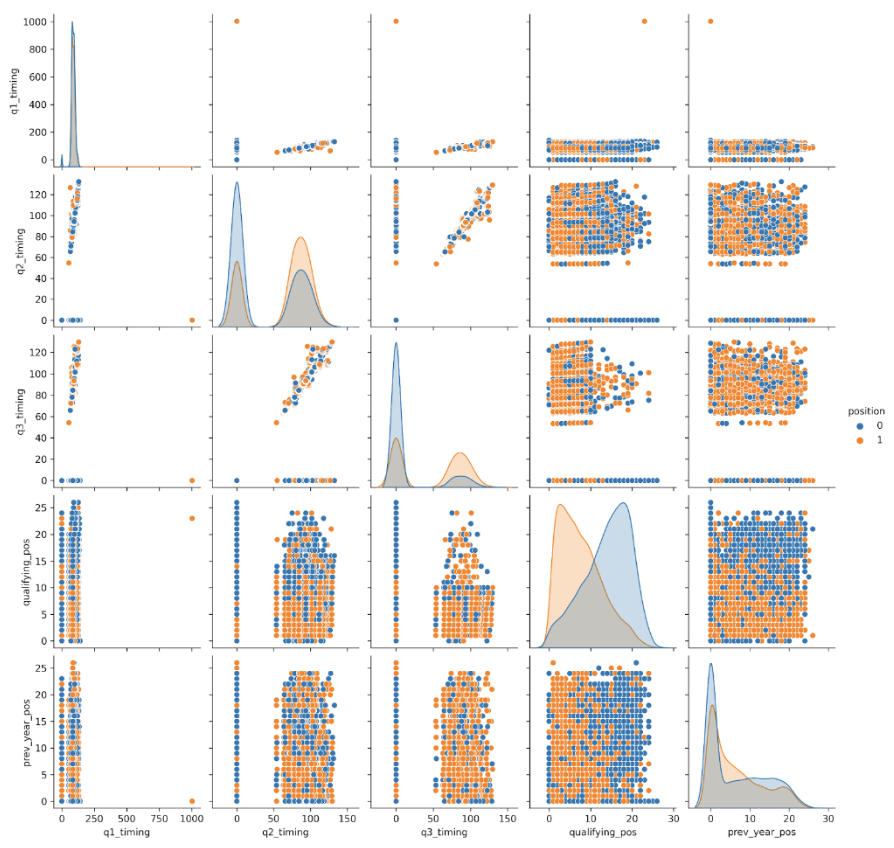
- Distinct Clusters in Timing Data: The scatter plots between
q2_timingandq3_timingdisplay distinct clusters, indicating that there may be distinct groups within the data. This could represent different performance tiers among the drivers or cars. - Positive Relationship between Q2 and Q3: There is a positive linear relationship between
q2_timingandq3_timing. Drivers who have lower (better) timings in Q2 also tend to have lower (better) timings in Q3. - Top 10 Finishers Distribution: When looking at the hue for
position, there appears to be a concentration of top 10 finishers (denoted by the color, possibly orange) with lowerqualifying_posvalues, reinforcing the importance of qualifying performance on race outcomes. - Timing and Qualifying Position: There is a trend visible in the scatter plots of the timing variables (q1_timing,
q2_timing,q3_timing) against qualifying_pos. Drivers with lower qualifying positions tend to have lower (faster) timings in all three qualifying sessions, particularly noticeable inq2_timingandq3_timing.
Feature Importance
A feature importance plot ranks the features of a model based on their importance in making accurate predictions, and in the context of a Random Forest Classifier, it reflects how much each feature contributes to reducing the variance in the model’s predictions.
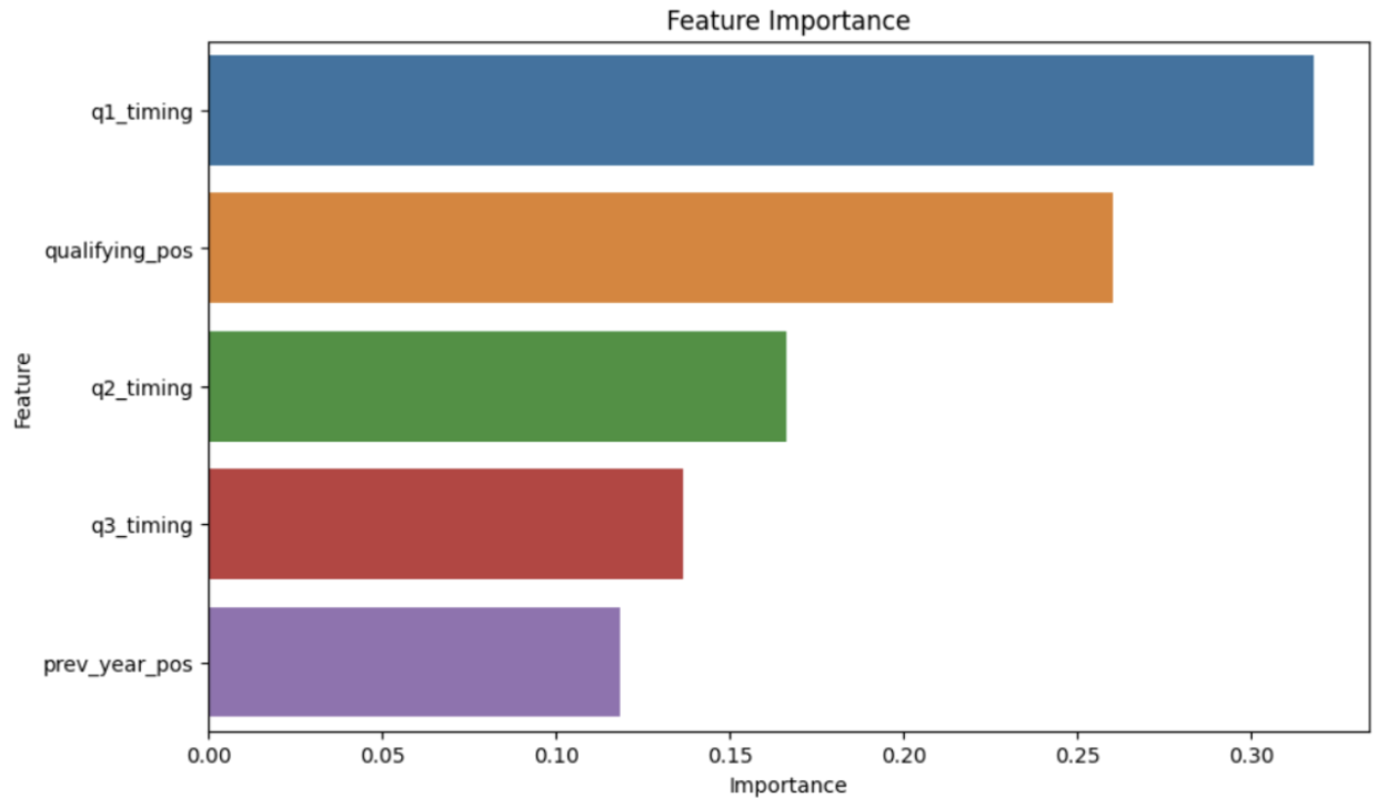
- Q1 Timing Dominance: The
q1_timingfeature has the highest importance score, suggesting it is the most significant predictor in determining the race position. - Lower Importance of Previous Year Position: The
prev_year_posfeature has the lowest importance score, indicating that it has the least influence on the model’s predictions of race position outcomes compared to the other features in the dataset.
Feature Engineering
Top 10 predictions
Track Clustering
Because clustering and dimensionality reduction algorithms require numeric representations of data, our categorical features were one-hot encoded. This transformation allowed us to integrate categorical and continuous data, enhancing the robustness of our analysis. Furthermore, to ensure features with larger scales did not dominate the cluster distance calculations, potentially biasing the clustering outcome, we leveraged a standard scaler to ensure that each feature contributes equally to the distance computations.
Modeling
Top 10 Predictions
Supervised learning is at the core of our project, focusing on predicting the likelihood of Formula 1 drivers finishing in the top 1 — an outcome critical for championship points. Our methodology involves training models on a dataset featuring variables such as track type, drivers’ past performances, qualifying positions, and lap times. The goal is to classify each race outcome into a binary variable indicating whether a driver finishes in the top 10. This focus is driven by the significant impact these positions have on championship standings.
We employ various models, including Random Forest, Logistic Regression, and Neural Networks, each chosen for its ability to capture different aspects of the complex dynamics influencing Formula 1 race outcomes. These models are trained, validated, and tested on data from the Ergast Developer API, providing a robust foundation for our predictive analysis. Accuracy is our primary metric for evaluating model performance, as it offers clear interpretability for our binary classification task, simplifying the analysis by focusing on the overall goal of identifying drivers and conditions that frequently lead to top 10 finishes.
Logistic Regression
Logistic Regression is a statistical method used to predict a binary outcome based on one or more predictor variables. It is particularly popular for binary classification tasks, such as predicting whether a driver will finish in the top 10.
Click here to see the code block
The function below was used to find the ideal the logistic regression model using grid search.
The provided code defines a function to construct and fine-tune a logistic regression model using grid search to explore a defined space of hyperparameters. GridSearchCV fits the model on the scaled training data using combinations of regularization strength (C), penalty type (penalty), and solver algorithm (solver) to determine the most effective parameters. The optimal model, with an l1 penalty, a regularization strength of 0.01, and the liblinear solver, achieved a prediction accuracy of 73.14% on the test dataset.
Random Forest
Random Forest is an ensemble learning method that constructs multiple decision trees and outputs the mode of the classes for classification tasks. It is known for its accuracy, robustness, and ability to handle large datasets with high dimensionality, reducing the risk of overfitting.
Click here to see the code block
The provided code builds and evaluates a Random Forest classifier using a grid search over specified hyperparameters. GridSearchCV systematically tests parameter combinations, cross-validating to find the best performance in terms of accuracy. The optimal model achieved an accuracy of 73.87% on the test set, with 200 trees (n_estimators), a maximum depth of 10 (max_depth), and a minimum split size of 10 (min_samples_split).
Neural Networks
Neural Networks are algorithms modeled after the human brain, designed to recognize patterns and perform classification tasks. They process information in a layered structure of nodes, making them effective for complex pattern recognition and predictive modeling.
Click here to see the code block
The provided code builds and optimizes a neural network model for binary classification using Keras and TensorFlow. A function, create_model, defines a neural network with one hidden layer and a given learning rate. The build_best_neural_network_model function uses GridSearchCV to iterate over hyperparameters such as the number of hidden nodes, learning rate, epochs, and batch size. The best-performing model, with 10 hidden nodes, a learning rate of 0.01, a batch size of 32, and training for 50 epochs, achieved an accuracy of 73.82% on the scaled test data.
Sensitivity Analysis
The sensitivity analysis across all three models — Random Forest, Logistic Regression, and Neural Network — reveals consistent findings. The feature qualifying_pos exhibits the highest sensitivity, indicating a strong influence on the model’s predictions; changes in qualifying position are likely to have a significant impact on the probability of a driver finishing in the top 10. In contrast, prev_year_pos shows notably lower sensitivity, suggesting that a driver’s position in the previous year is less indicative of their performance in the current race. The timing features (q1_timing, q2timing, q3_timibg) demonstrate moderate sensitivity, with some variability across the models, reflecting their respective influence on race outcomes. This consistent pattern across different models underscores the robustness of these features’ influences on predicting top 10 finishes in Formula 1 races.
Click here to see the code block
Failure Analysis
Supervised learning, while a powerful tool for predictive modeling, may encounter significant challenges in the context of Formula 1 race outcome predictions, primarily due to the intricacies and complexities inherent to the sport. One of the fundamental hurdles is the inadequacy of available data concerning the detailed specifications and configurations of F1 cars. This information, encompassing aspects like downforce levels, ground clearance, engine settings, and more, remains proprietary to each racing team. Such data is critical for accurately forecasting race outcomes, as these variables can significantly impact a car’s performance on different tracks under varying conditions. Moreover, the dynamic nature of F1 races, where strategies and car setups are meticulously tailored for each race weekend, further complicates the predictive modeling efforts. Without access to this depth of data, supervised learning models are limited to more surface-level features, potentially overlooking nuanced factors that are decisive for race results.
Additionally, our approach deliberately excludes pit stop strategies from the predictive factors, considering them as in-race variables that are not predetermined and thus fall outside the scope of pre-race predictions. This decision, while simplifying the modeling process, omits a crucial element of race strategy that can dramatically influence race outcomes. Pit stops are often used strategically to gain an advantage over competitors, and their timing and execution can vary based on a multitude of factors, including weather conditions and tire performance. Furthermore, the unpredictable nature of mechanical failures and retirements adds another layer of complexity to race outcome predictions. Cars may fail for myriad reasons, from engine blowouts to collisions, which are virtually impossible to predict with supervised learning models based solely on historical data. These elements introduce a level of randomness and uncertainty that can derail even the most sophisticated models, underscoring the limitations of using supervised learning for predicting outcomes in a sport as complex and multifaceted as Formula 1.
Track Clustering
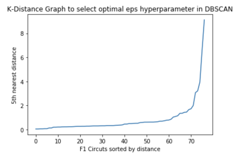
Our primary clustering algorithm was DBSCAN (Density-Based Spatial Clustering of Applications with Noise). This unsupervised clustering algorithm is known for its efficacy in identifying non-normally distributed clusters of varying shapes and sizes without predefining the number of clusters. The optimal epsilon value, a critical hyperparameter for DBSCAN, was estimated using the Nearest Neighbors algorithm. We adhered to the heuristic of setting n_neighbors to 2*dim - 1, where dim represents the dimensionality of our feature space, to balance local density estimation and computational feasibility. We determined the optimal epsilon value by evaluating where the distance of the 5th nearest neighbor stated to increase exponentially in the K-distance graph.
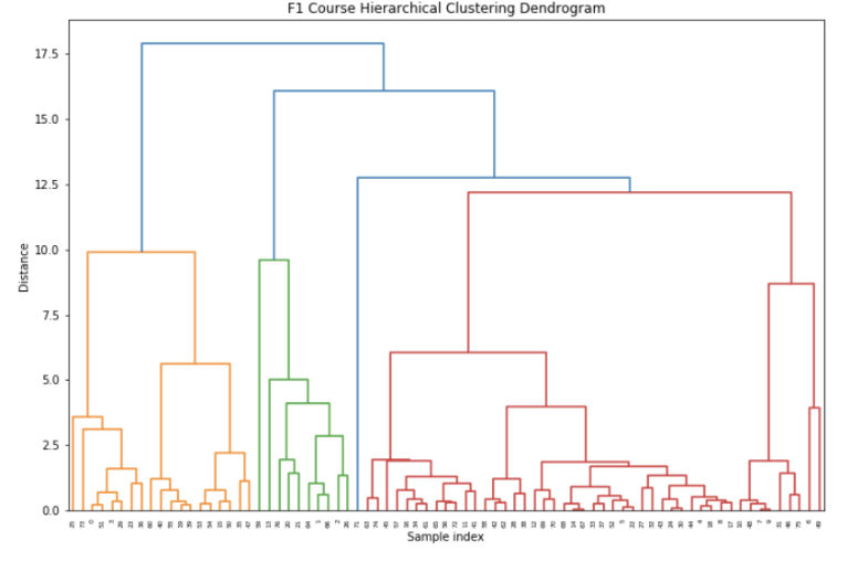
Simultaneously, we explored hierarchical clustering to validate our findings with DBSCAN. Through visual inspection of a dendrogram, we optimized the distance threshold to ensure that there was significant dissimilarity between clusters. Despite some variance, both DBSCAN and hierarchical clustering revealed similar cluster structures, underscoring the generalizability of the clusters produced by DBSCAN.
To evaluate the sensitivity of our clusters to changes in the data, we took three bootstrap random samples of 80% of the data. These bootstrap samples yielded similar clusters to clusters generated from the entire dataset, denoting the stability of our clustering approach to changes in the data.
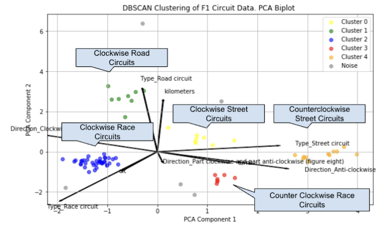
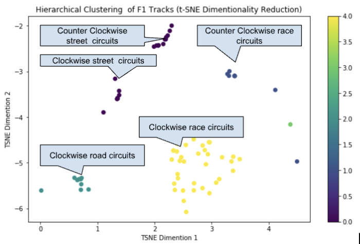
To navigate the high-dimensional nature of our data, we leveraged Principal Component Analysis (PCA) and t-Distributed Stochastic Neighbor Embedding t-SNE for dimensionality reduction to visualize in two-dimensions. While PCA provided a broad overview of data variance, t-SNE allowed us to observe the nuanced structure of our clusters in two dimensions. Our biplot overlay on the PCA scatter plot revealed that circuit types and directions were predominant drivers behind the clustering.
Discussion
Top 10 Prediction
The Random Forest model, with its ensemble approach, provided an accuracy of 73.87%, indicating a robust predictive capability potentially due to its handling of non-linear relationships between features and the target variable. This model’s performance was slightly outperformed by the Neural Network model, which achieved an accuracy of 73.82%, with an architecture of a single hidden layer containing ten nodes. The Neural Network’s performance, despite being marginally lower, suggests that a more complex model does not necessarily guarantee superior results, considering the computational complexity and time taken to train such models. The Logistic Regression model, a more straightforward and interpretable model, yielded a slightly lower accuracy of 73.14%. This could be attributed to its linear nature, which may not capture complex patterns in the data as effectively as the other two models. However, the difference in accuracy is relatively small, highlighting that simpler models can still be competitive and beneficial, especially when considering the trade-off between performance and model complexity.
The feature importance plot and the pair plot provided valuable insights into the predictive power of different features, with q1_timing and qualifying_pos being the most significant predictors across models, aligning with domain knowledge that qualifying performances have substantial impacts on race outcomes. The negligible importance of the prev_year_pos feature suggests that past performance is not a reliable indicator of future race results, pointing to the dynamic nature of the sport where numerous variables can influence race day performance.
Track Clustering
In our unsupervised analysis of clustering Formula 1 circuits, tuning hyperparameters in the DBSCAN algorithm emerged as a significant factor in achieving meaningful clusters. This aspect underscores that adjustment of algorithm parameters can profoundly impact the outcomes and interpretability of the results. However, we encountered a remarkable challenge when categorical variables, rather than continuous variables like track length, number of turns, and altitude, predominantly drove the variation in clusters. This observation was somewhat anticipated, given the relative uniformity in these continuous variables across different tracks, which consequently led to categorical factors becoming more influential in the clustering process. This outcome, while initially disappointing, provided valuable insights into the feature space of track characteristics. In light of these findings, future work should pivot towards exploring the clustering of driver finish times in relation to track characteristics. This direction aims to delve deeper into the potential correlations between track features and performance outcomes, potentially uncovering patterns that could inform strategic decisions in race preparation and execution.